Represents EDR trajectories in the state space. Trajectories and/or states can be displayed in different colors based in a predefined classification or variable.
Usage
plot_edr(
  x,
  trajectories,
  states,
  traj.colors = NULL,
  state.colors = NULL,
  variable = NULL,
  type = "trajectories",
  axes = c(1, 2),
  initial = F,
  ...
)
Arguments
- x
Symmetric matrix or
distobject containing the dissimilarities between each pair of states of all trajectories in the EDR. Alternatively, data frame containing the coordinates of all trajectory states in an ordination space.- trajectories
Vector indicating the trajectory or site to which each state in
xbelongs.- states
Vector of integers indicating the order of the states in
xfor each trajectory.- traj.colors
Specification for the color of all individual trajectories (defaults "grey") or a vector with length equal to the number of different trajectories indicating the color for each individual trajectory.
- state.colors
Specification for the color of all trajectory states (defaults equal to
traj.colors), vector with length equal to the number of states indicating the color for each trajectory state, or vector of colors used to generate a gradient depending on the values ofvariable(iftype = "gradient").- variable
Numeric vector with equal length to the number of states to be represented using a gradient of state colors (if
type = "gradient").- type
One of the following
"trajectories","states", or"gradient".- axes
An integer vector indicating the pair of axes in the ordination space to be plotted.
- initial
Flag indicating if the initial state must be plotted (only if
type = "states"ortype = "gradient")- ...
Arguments for generic
plot().
Value
plot_edr() permits representing the trajectories of an Ecological Dynamic
Regime using different colors for each trajectory or state.
See also
plot.RETRA() for plotting representative trajectories in an ordination space
representing the state space of the EDR.
Examples
# Data
state_variables <- EDR_data$EDR1$abundance
d <- EDR_data$EDR1$state_dissim
# Coordinates in classic multidimensional scaling
x <- cmdscale(d, k = 3)
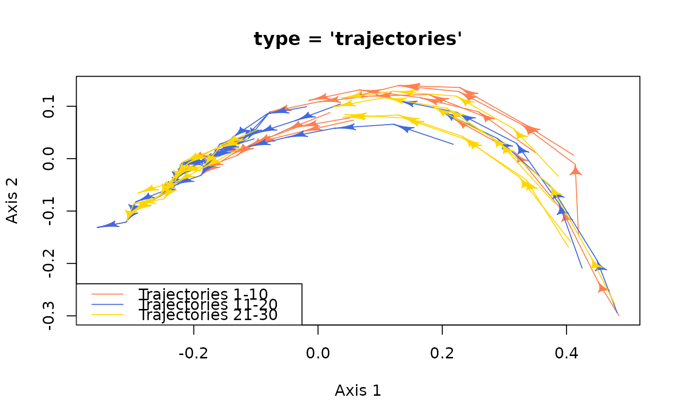
# Plot trajectories 1-10 in "coral", 11-20 in "blue" and 21-30 in "gold"
plot_edr(x = x, trajectories = state_variables$traj,
states = as.integer(state_variables$state),
traj.colors = c(rep("coral", 10), rep("royalblue", 10), rep("gold", 10)),
xlab = "PCoA 1", ylab = "PCoA 2",
main = "type = 'trajectories'")
legend("bottomleft", legend = paste0("Trajectories ", c("1-10", "11-20", "21-30")),
lty = 1, col = c("coral", "royalblue", "gold"), bty = "n", cex = 0.9)
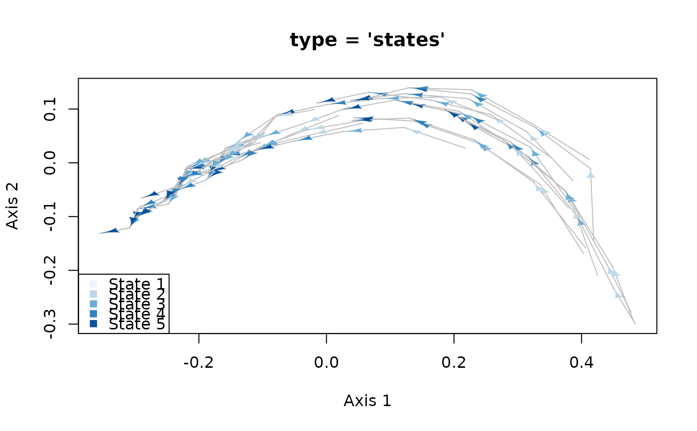
 # Plot states with different colors depending on the state value
plot_edr(x = x, trajectories = state_variables$traj,
states = as.integer(state_variables$state),
traj.colors = NULL, initial = TRUE,
state.colors = rep(c("coral2", "azure3", "azure3", "azure3", "royalblue4"),
length(unique(state_variables$traj))),
xlab = "PCoA 1", ylab = "PCoA 2",
type = "states", main = "type = 'states'")
legend("bottomleft", legend = c("State 1", "States 2-4", "State 5"),
pch = 15, col = c("coral2", "azure3", "royalblue4"), bty = "n", cex = 0.9)
# Plot states with different colors depending on the state value
plot_edr(x = x, trajectories = state_variables$traj,
states = as.integer(state_variables$state),
traj.colors = NULL, initial = TRUE,
state.colors = rep(c("coral2", "azure3", "azure3", "azure3", "royalblue4"),
length(unique(state_variables$traj))),
xlab = "PCoA 1", ylab = "PCoA 2",
type = "states", main = "type = 'states'")
legend("bottomleft", legend = c("State 1", "States 2-4", "State 5"),
pch = 15, col = c("coral2", "azure3", "royalblue4"), bty = "n", cex = 0.9)
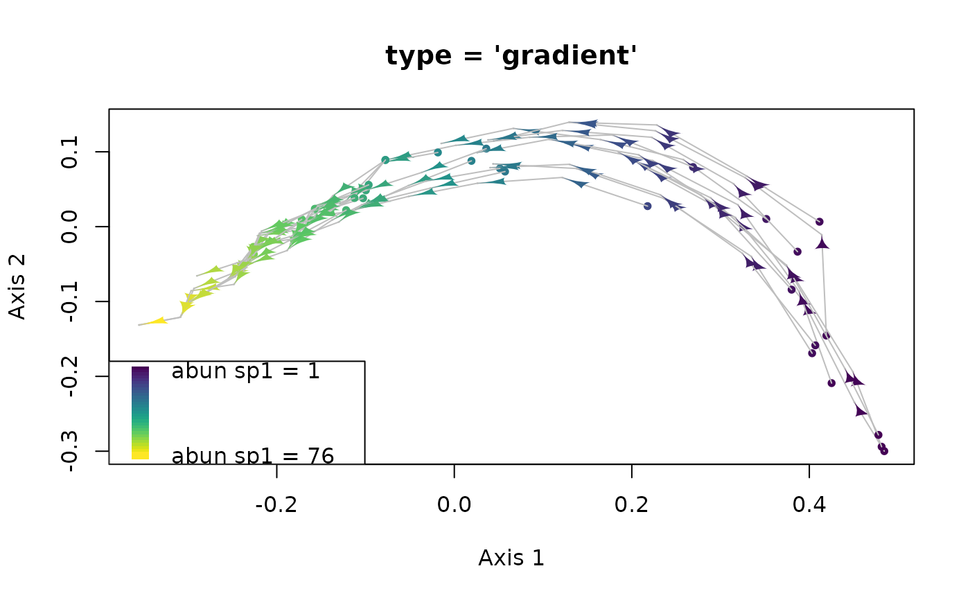
 # Plot states with different colors depending on the abundance of sp1
plot_edr(x = x, trajectories = state_variables$traj,
states = as.integer(state_variables$state),
traj.colors = NULL,
state.colors = c("yellow", "orange2", "purple4"),
variable = state_variables$sp1,
xlab = "PCoA 1", ylab = "PCoA 2",
type = "gradient", main = "type = 'gradient'", initial = TRUE)
legend("bottomleft",
legend = c(paste0("abun sp1 = ", min(state_variables$sp1)),
rep(NA, 28),
paste0("abun sp1 = ", max(state_variables$sp1))),
fill = colorRampPalette(c("yellow", "orange2", "purple4"))(30),
border = NA, y.intersp = 0.2, cex = 0.9, bty = "n")
# Plot states with different colors depending on the abundance of sp1
plot_edr(x = x, trajectories = state_variables$traj,
states = as.integer(state_variables$state),
traj.colors = NULL,
state.colors = c("yellow", "orange2", "purple4"),
variable = state_variables$sp1,
xlab = "PCoA 1", ylab = "PCoA 2",
type = "gradient", main = "type = 'gradient'", initial = TRUE)
legend("bottomleft",
legend = c(paste0("abun sp1 = ", min(state_variables$sp1)),
rep(NA, 28),
paste0("abun sp1 = ", max(state_variables$sp1))),
fill = colorRampPalette(c("yellow", "orange2", "purple4"))(30),
border = NA, y.intersp = 0.2, cex = 0.9, bty = "n")